こんにちは。次世代システム研究室のK.S.（女性、外国人）です。

最近は桜の季節も終わり、新しく夏の自然や緑に触れたくなりませんでしょうか。常夏の国で生まれた私はいつも日本の季節変化を楽しみにしています。それを言い訳にして、平日の渋谷出勤を離れて、日本の自然を味わうため、大山へ山登りに行ってきました。登っていると、水の音が聞こえてきて、池があるのかなと感じました。音の方に向かって、近くまで行ったら、おっと、池ではなく、滝でした。あらあら、自分の耳はきちんと池と滝を判別できないのかちょっとびっくりしました。そこで、自分の耳の代わりに音を分類するものがあればいいなあと思って、音を分類してみたいと考えました。一応、遊んでばかりではいけないので、ついでに自分が遊べるネタに関係がある技術も少し紹介できればと思います。そこで、最近の機械学習分野で注目されていて、かつ、音の分類にも役に立ちそうな技術を取り上げることにしました。

最近、機械学習分野がすばやい広がりを見せています。多くのデータセットが公開され、それらのデータを利用し、様々な学習モデルが作成されています。特に、画像認識分野では ResNet, VGG, AlexNetといった様々な条件での学習されたモデルが沢山公開されています。また、自然言語処理分野でも、去年から話題になったモデルがたくさん公開されています。去年、GoogleのAIチームがBERTというモデルを発表し、今年もBERTを越えたXLNet モデルを発表しました。さらに、今年MicrosoftがMT-DNNを発表しました。学習モデルが自由に使えるようになったおかげで、高いコストと長い時間をかけて苦労してモデルを作る必要が少なくなってきています。そこで、今回は、転移学習（Transfer learning）という技術について書かせて頂こうと思います。転移学習とはなにか、学習済みモデルがあると転移学習になにに役に立つのか、基礎から深くまで勉強するため、会社のスキルアップ支援でhands-on transfer learning with python の本を購入しました。今回の説明は主にこの本とこのサイトを参考にしています。

さて、今回のブログは自分の遊び8割と勉強2割を合わせて、転移学習についての情報を共有し、この技術を使って池と滝の音を予測してみたいと思います。このブログの構成は、以下のとおりです。

①　転移学習（transfer learning）とは
②　音声分類：池と滝の音の予測
③　まとめと考察

① 転移学習（transfer learning）とは

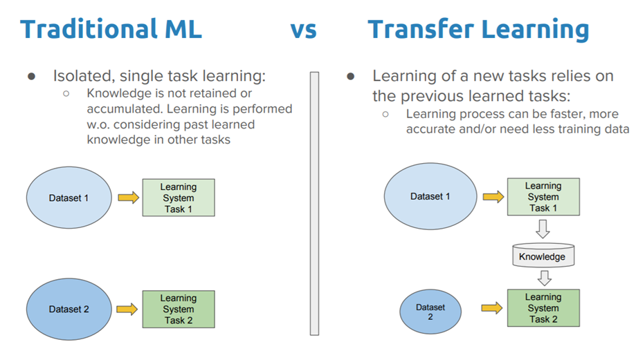
転移学習（Transfer learning）はあるタスクで学習されたモデルを他のタスクに適応することです。わかりやすくするため、人の学習の仕方を例にします。ある人が子供のときに、泳ぎ方を学びました。大人になって、ダイビングを学びたいときに、ゼロから学習しなくても、泳ぎ方を知っているので、それを活かして、ダイビングを学びます。水泳とダイビングはまったく同じ知識ではないですが、部分の知識を活かしながら学習することが転移学習です。機械学習の話に戻ると、従来の機械学習は一つのデータセットを使って学習し、学習モデルを作成します（図１）。二つのタスクだと、二回学習する必要があります。そうすると、特定タスクのためにたくさん学習データが必要で学習時間もかかります。この課題を改善するため、転移学習は人間の学習の仕方を真似て、学習したことがあるタスクの知識を別のタスクに活かしながら、学習します。結果、ゼロから学習する必要がないから、最初の学習ベースラインの性能を高めることができ、学習時間を節約することもできます。さらに、様々なノウハウを活かすため、最終的な学習精度も期待できます。

 

図１：転移学習（Transfer learning）のイメージこのサイトより転載 

転移学習の戦略

このセクションでは転移学習の定義を説明させていただきます。このセクションを読む前に、少し確率論を復習して頂ければわかりやすくなるかと思います。

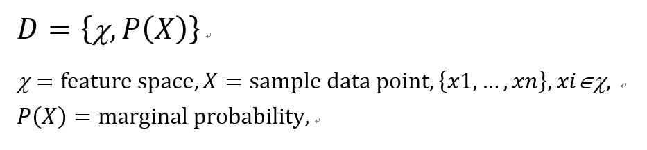
domain（Ｄ）は二つの構成要素（feature spaceとmarginal probability）からなる組と定義されています。

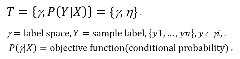
タスク（T）二つの構成要素（label spaceとobjective function）からなる組と定義されています。

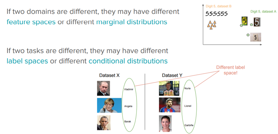
ここで、objective functionは featureとlabelから学習することになります。すると、転移のタスクは4つのシナリオ「feature space、marginal probability、label space、conditional probabilities」を含まれます。どこのsourceとtargetが異なるのか、転移学習が変わっていきます（図2）。

 

図１：転移学習定義のイメージこのサイトより転載 

さて、転移学習を行うためには、なに（What）、いつ(When)、どうやって(How)、転移するのか答えるのが必要です。まず、何を転移するのかが一番大事です。知りたい答えを明らかにするため、転移学習は知識を転移します。そこで、どこから（ソース）、どこまで（ターゲット）が共通知識かを識別することが必要です。それから、知識を転移するのがいつもよい方向の結果を与えるわけではなく、悪い転移になる可能性もあります。何を転移すべきで何を転移すべきでないかは注意が必要です。最後に、転移学習は既存アルゴリズムや手法を修正します。どの部分に転移手法を入れるべきなのかきちんとと特定するのが必要です。

転移学習の手法

上記に記したように、たくさん学習モデルができてきて、転移学習の応用が広がってきました。それらの学習モデルはだいたいディープラーニング（従来の機械学習アルゴリズム）モデルですので、ここでは、ディープラーニングにおける、転移学習の手法に注目させていただきます。転移学習の手法は主に二つに分かれ、feature-extraction(特徴抽出)とfine-tuning（微調整）です。

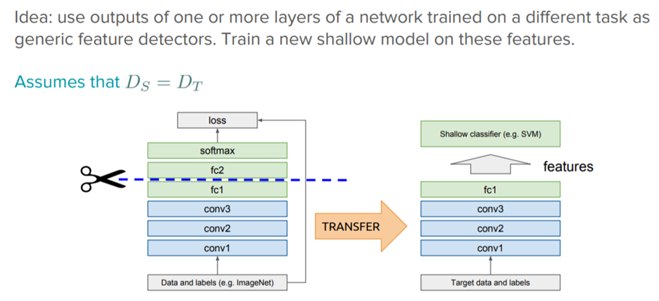
feature-extraction (特徴抽出)

ディープラーニングのシステムとモデルは、様々な特徴（feature）を学習する階層化アーキテクチャーです。転移学習のfeature-extractionはこのネットワーク構想を利用します。例えば、ディープラーニングモデルは、モデルを作成するときに、様々な層を通じで学習を行います。転移学習は学習済みモデルの情報（いくつかの層）を転移し、別のタスクのための新しいモデルを作成します。例として、図2のように、学習済みのモデルのconv1層からfc1層までを転移します。その部分は学習済みなので、もう一度学習する必要なく、feature情報として利用します。それらのfeatureを新しい別の層と繋いで、出力層を作成し、モデルを作ります。事前に学習されたモデルの最後の層は他のタスクのfeature extractorになります（図２）。

 

図２：feature-extractionのイメージこのサイトより転載 

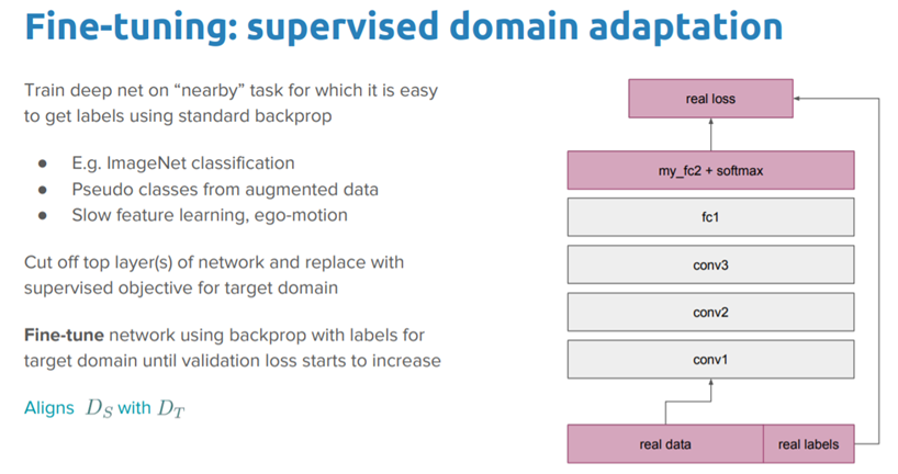
fine-tuning（微調整）

最後の層を入れ替えるだけではなく、前のレイヤーも再学習できます。これがfine-tuningです（図３）。

 

図3：fine-tuningのイメージこのサイトより転載 

現在、ディープラーニングは、移転学習が応用されているアルゴリズムの一種です。応用は主に3つの分野に分かれていて、テキストデータの転移学習、コンピュータビションの転移学習、音声の転移学習です。今回のブログの実験では転移学習を用いての音の分類を試します。

それでは、お待たせしました。長い説明になってしまいましたが、いよいよ、実装が始まります。

② 音声分類：池と滝の音の予測

それでは、転移学習を使って、池と滝の音を分類し、音を予測したいと思います。実装の詳細はJupyter notebookの中で説明していますので、ご参考にして頂ければと思います。また、Jupyter notebookはgithubからダウンロード可能です。

いよいよ、実装開始です。

今回の転移学習はConvolutional Neural Network(畳み込みニューラルネットワーク、以下CNN)を適応します。CNNは画像処理でよく使われますので、沢山な学習済みモデルが公開されています。そのモデルを使って、転移学習を適用し、音を分別します。CNNを使いやすくするため、音を画像に変換して利用します。

データ準備

データ処理の詳細は、Jupyter notebookを参考にして下さい。

まず、youtube_dlモジュールを使って、youtubeからmp3で池と滝の音声データをダウロードします。

from __future__ import unicode_literals
import youtube_dl

# download audio files from youtube
def download_youtube_file(output_filename, download_link):
    ydl_opts = {
        'format': 'bestaudio/best',
        'postprocessors': [{
            'key': 'FFmpegExtractAudio',
            'preferredcodec': 'mp3',
            'preferredquality': '192'            
        }],
        'outtmpl': output_filename+'.%(ext)s'
    }
    with youtube_dl.YoutubeDL(ydl_opts) as ydl:
        ydl.download([download_link])
    return
    
download_youtube_file("waterfall_1", "https://www.youtube.com/watch?v=OnMjo-CoOg8")    
download_youtube_file("waterfall_2", "https://www.youtube.com/watch?v=EoLhnbsWsOY")  
download_youtube_file("waterfall_3", "https://www.youtube.com/watch?v=FF2bhR7s3VY")  
download_youtube_file("pond_1", "https://www.youtube.com/watch?v=6VZxnWZcYLM")
download_youtube_file("pond_2", "https://www.youtube.com/watch?v=UN5hyc6OTX8")
download_youtube_file("pond_3", "https://www.youtube.com/watch?v=yYCqZSEtXiY")

これらの音mp3ファイルをwavファイルに変換し、音の長さを調整します。

from pydub import AudioSegment
import os

# generate small audio files from the downloaded youtube files
def generate_small_audio_files(filename):
    mp3_file = filename+".mp3"
    sound = AudioSegment.from_mp3(mp3_file)
    sound.export(filename+".wav", format="wav")

    if not os.path.exists('audio_files'):
        os.makedirs('audio_files')
        
    count=1
    for i in range(1,1000,15):
        if count>50:
            break
        t1 = i * 1000 # in milliseconds
        t2 = (i+15) * 1000
        newAudio = AudioSegment.from_wav(filename+".wav")
        newAudio = newAudio[t1:t2]
        newAudio.export('audio_files/'+filename+"_"+str(count)+'.wav', format="wav")
        count+=1
    print (filename, count)
    return
generate_small_audio_files("waterfall_1")
generate_small_audio_files("pond_1")
generate_small_audio_files("waterfall_2")
generate_small_audio_files("pond_2")
generate_small_audio_files("waterfall_3")
generate_small_audio_files("pond_3")

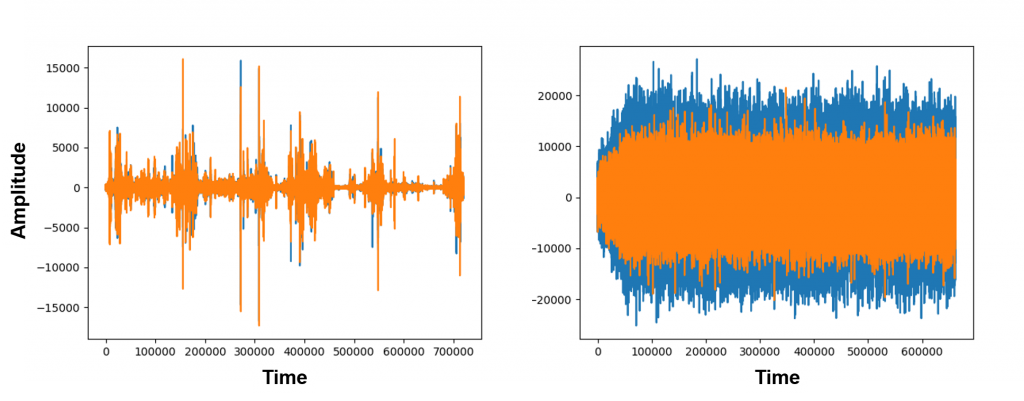
次に、CNNの画像モデルを適応するため、音ファイルを画像に変換します。wavファイルから画像に変化します。変換形はwaveとspecgramを変換してみました。しかし、今回の実験はwave系のみを用いて行いました。

waveの変換ファイルの例です。

import os
from os import walk
from scipy.io.wavfile import read
import matplotlib.pyplot as plt

# convert audio files to wave figures
def convert_audio_to_wave(_name):
    if not os.path.exists("fig_wave"):
        os.makedirs("fig_wave")
    thing_wavs = []
    for (_,_,filenames) in walk("audio_files"):
        thing_wavs.extend(filenames)
        break
    for thing_wav in thing_wavs:
        input_data = read("audio_files/" + thing_wav)
        audio = input_data[1]
        f = plt.figure()
        plt.plot(audio)
        plt.ylabel("Amplitude")
        plt.xlabel("Time")
        plt.savefig("fig_wave/" + thing_wav.split('.')[0] + '.png')
        if thing_wav ==_name+"_1.wav":
            plt.show()
        f.clear()
        plt.close(f)
    return
convert_audio_to_wave("waterfall_1")
convert_audio_to_wave("pond_1")
convert_audio_to_wave("waterfall_2")
convert_audio_to_wave("pond_2")
convert_audio_to_wave("waterfall_3")
convert_audio_to_wave("pond_3")

図4：Wave形に変換した例「左は池、右は滝」 

specgramの変換ファイルの例です。

# convert audio files to specgram figures
def convert_audio_to_specgram(_name):
    if not os.path.exists("fig_specgram"):
        os.makedirs("fig_specgram")
    thing_wavs = []
    for (_,_,filenames) in walk("audio_files"):
        thing_wavs.extend(filenames)
        break
    for thing_wav in thing_wavs:
        samplingFrequency, signalData = read("audio_files/" + thing_wav)
        input_data = read("audio_files/" + thing_wav)
        f = plt.figure()
        plt.specgram(signalData[:,0], Fs=samplingFrequency)
        plt.ylabel("Frequency")
        plt.xlabel("Time")
        plt.savefig("fig_specgram/" + thing_wav.split('.')[0] + '.png')
        if thing_wav ==_name+"_1.wav":
            plt.show()
        f.clear()
        plt.close(f)

convert_audio_to_specgram("waterfall_1")
convert_audio_to_specgram("pond_1")
convert_audio_to_specgram("waterfall_2")
convert_audio_to_specgram("pond_2")
convert_audio_to_specgram("waterfall_3")
convert_audio_to_specgram("pond_3")

図５：Specgram形に変換した例「左は池、右は滝」 

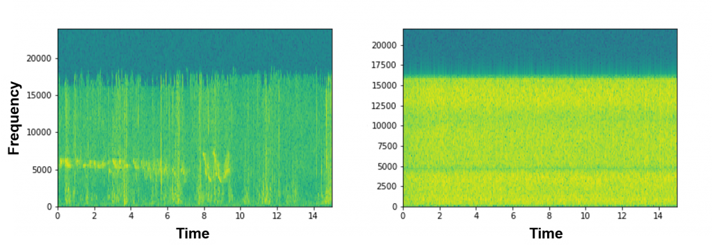
図を見ても、池と滝のイメージが結構違うのがわかります。これらの図を見ると、少し池と滝の音を識別できる可能性を感じてきました。

転移実験

それでは、準備した画像データを使って、転移学習の実験を行いたいと思います。今回、やってみたいことは３つの学習方法（上記に説明した転移学習のfeature extractionとfine tuning（簡単版）と転移学習なしでのCNN）を使って、池と滝の音が変換された画像を学習してみます。それから、それぞれの学習モデルを使って、音の識別をしてみます。実装コードはこのリンクになります。

 

トレーニングデータとテストデータ分け

データはトレーニング（学習のためのデータ）とテスト(学習モデルを使ってテストするためのデータ)に分けて実験します。トレーニングデータは「転移学習：feature extractionでの学習」、「転移学習：fine tuningでの学習」、「転移学習なしで、CNNでの学習」で利用します。テストデータは「音声の予測」で利用します。

import glob
import numpy as np
import matplotlib.pyplot as plt
from sklearn.model_selection import train_test_split
from sklearn.preprocessing import LabelEncoder
from keras.preprocessing.image import ImageDataGenerator, load_img, img_to_array, array_to_img
%matplotlib inline

IMG_DIM = (150, 150)

# Load image and covert to numpy array
all_files = glob.glob('fig_wave/*')
# all_files = glob.glob('fig_specgram/*')
all_imgs = [img_to_array(load_img(img, target_size=IMG_DIM)) for img in all_files]
all_imgs = np.array(all_imgs)
all_labels = [fn.split('\\')[1].split('.')[0].split('_')[0].strip() for fn in all_files]

# Seperate train, validation, and test datasets
train_imgs, not_train_imgs, train_labels, not_train_labels = train_test_split(all_imgs, all_labels, test_size=0.5, random_state=42)
validation_imgs, test_imgs, validation_labels, test_labels = train_test_split(not_train_imgs, not_train_labels, test_size=0.5, random_state=42)

# Scale the images
train_imgs_scaled = train_imgs.astype('float32')
validation_imgs_scaled  = validation_imgs.astype('float32')
test_imgs_scaled = test_imgs.astype('float32')
train_imgs_scaled /= 255
validation_imgs_scaled /= 255
test_imgs_scaled /= 255

# Set up parameters for training
batch_size = 30
num_classes = 2
epochs = 30
input_shape = (150, 150, 3)

# Encode text to labels
le = LabelEncoder()
le.fit(train_labels)
train_labels_enc = le.transform(train_labels)
validation_labels_enc = le.transform(validation_labels)
test_labels_enc = le.transform(test_labels)

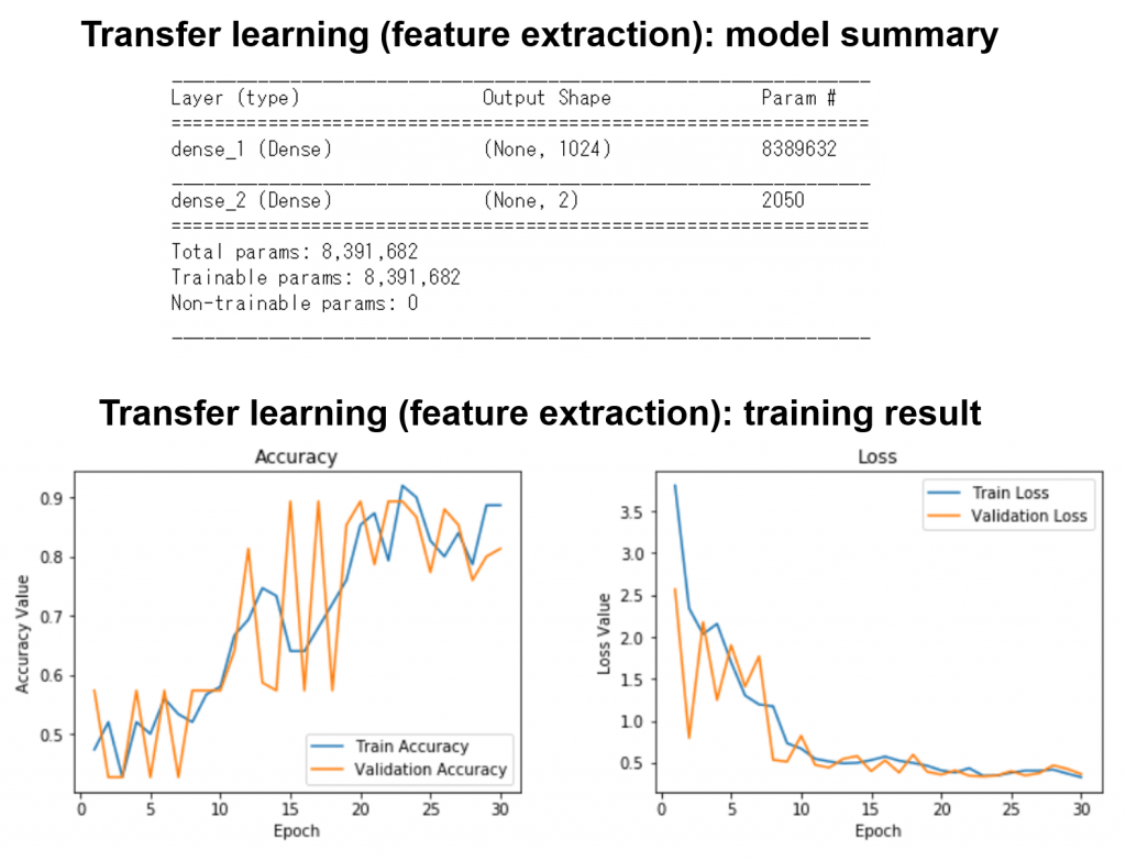
転移学習：feature extractionでの学習

学習モデル（pretrained CNN model）をfeature extractorとして学習します（図２）。学習済みモデルVGG16を使いました。

import os
import numpy as np
from keras.applications.vgg16 import VGG16,preprocess_input,decode_predictions
from keras.preprocessing import image
from keras.models import Model
from keras import layers
from keras.applications.imagenet_utils import preprocess_input
from keras.utils import to_categorical
from keras.models import Sequential
from keras import optimizers, losses
from keras import layers

# Get pretrained model (vgg16) for transfer learning
vgg16 = VGG16(include_top=False, weights='imagenet', input_shape=input_shape)

# Remove the last layer of the pretrained model
output = vgg16.layers[-1].output
output = layers.Flatten()(output)

# Freeze the model which will be extracted as a feature later
vgg16_model = Model(vgg16.input, output)
vgg16_model.trainable = False	

# Show a summary of the pretrained model. Check the number of trainable parameters
vgg16_model.summary()

# Create functions for feature extraction
def extract_tl_features(model, base_feature_data):
    dataset_tl_features = []
    for index, feature_data in enumerate(base_feature_data):
        if (index+1) % 1000 == 0:
            print('Finished processing', index+1, 'sound feature maps')
        pr_data = process_sound_data(feature_data)
        tl_features = model.predict(pr_data)
        tl_features = np.reshape(tl_features, tl_features.shape[1])
        dataset_tl_features.append(tl_features)
    return np.array(dataset_tl_features)
def process_sound_data(data):
    data = np.expand_dims(data, axis=0)
    data = preprocess_input(data)
    return data

# Extract features from pretrained model (vgg16)
train_vgg16 = extract_tl_features(vgg16_model, train_imgs_scaled)
print (train_imgs_scaled.shape, train_vgg16.shape)
validatation_vgg16 = extract_tl_features(vgg16_model, validation_imgs_scaled)
test_vgg16 = extract_tl_features(vgg16_model, test_imgs_scaled)

# Convert a vector label to matrix label
train_labels_ohe = to_categorical(train_labels_enc)
validation_labels_ohe = to_categorical(validation_labels_enc)
test_labels_ohe = to_categorical(test_labels_enc)
print (train_labels_ohe.shape,train_labels_ohe.shape[0])

# Create the model
model2 = Sequential()

# Add new layers and pre-trained model (vgg16) as an input feature
model2.add(layers.Dense(1024, activation='relu', 
                       input_shape=(train_vgg16.shape[1],)))
model2.add(layers.Dense(train_labels_ohe.shape[1], activation='softmax'))

# Compile the model
model2.compile(loss='categorical_crossentropy', optimizer='adam',                 
                      metrics=['accuracy'])

# Show a summary of the model. Check the number of trainable parameters
model2.summary()

学習結果は下記になります。学習回数を増やすと、学習精度がどんどんよくなっていくことがみられました。学習がうまくできたことを確認できました。

図５：転移学習(feature extraction)の学習結果 

 

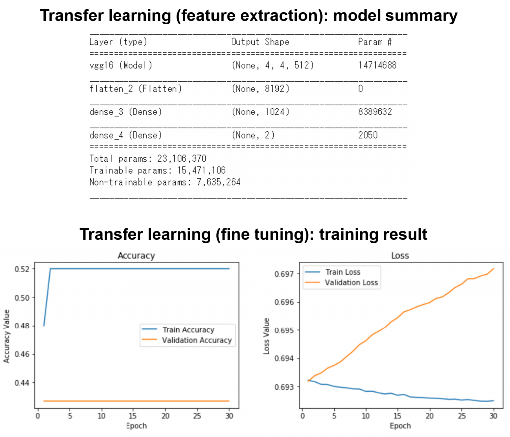
転移学習：fine tuningでの学習

学習モデル（pretrained CNN model）をfine tuningし、モデルを再学習します（図3）。学習済みモデルVGG16を使いました。

# Create the model
model3 = Sequential()
 
# Add the vgg convolutional base model
model3.add(vgg16_model2)
 
# Add new layers
model3.add(layers.Flatten())
model3.add(layers.Dense(1024, activation='relu'))
model3.add(layers.Dense(train_labels_ohe.shape[1], activation='softmax'))
model3.compile(loss='categorical_crossentropy', optimizer='adam',                 
                      metrics=['accuracy'])

# Show a summary of the model. Check the number of trainable parameters
model3.summary()

学習結果は下記になります。学習がなかなかうまく行きませんでした。

図6：転移学習(fine tuning)の学習結果 

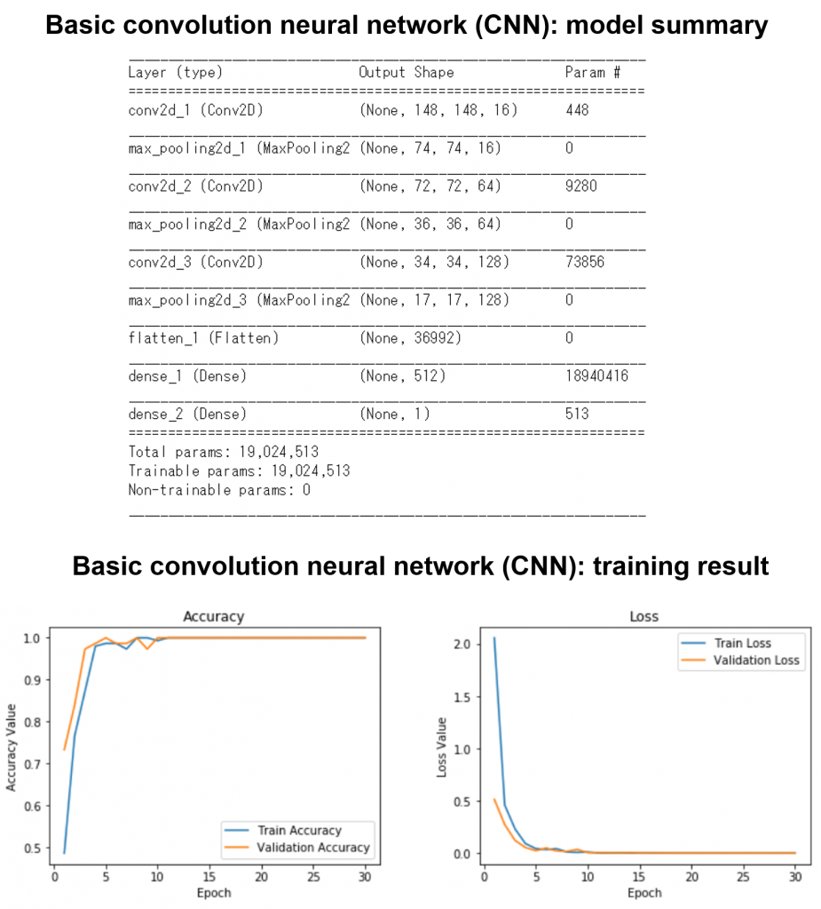
転移学習なしで、CNNでの学習

同じトレーニングデータを使ってCNNで学習ました。モデルは下記に載せていますが、詳細実装はjupyterファイルを参考にして下さい。

from keras.layers import Conv2D, MaxPooling2D, Flatten, Dense, Dropout
from keras.models import Sequential
from keras import optimizers, losses

# Create the model
model = Sequential()

# Add the CNN layers
model.add(Conv2D(16, kernel_size=(3, 3), activation='relu', input_shape=input_shape))
model.add(MaxPooling2D(pool_size=(2, 2)))
model.add(Conv2D(64, kernel_size=(3, 3), activation='relu'))
model.add(MaxPooling2D(pool_size=(2, 2)))
model.add(Conv2D(128, kernel_size=(3, 3), activation='relu'))
model.add(MaxPooling2D(pool_size=(2, 2)))
model.add(Flatten())
model.add(Dense(512, activation='relu'))
model.add(Dense(1, activation='sigmoid'))

# Compile the CNN model
model.compile(loss=losses.binary_crossentropy,optimizer=optimizers.adam(), metrics=['accuracy'])

# Show a summary of the model. Check the number of trainable parameters
model.summary()

結果、池と滝の音は100%特定できましたが、overfittingの可能性が高いです。

図7：転移学習なしで、Convolution neural network(CNN)での学習結果 

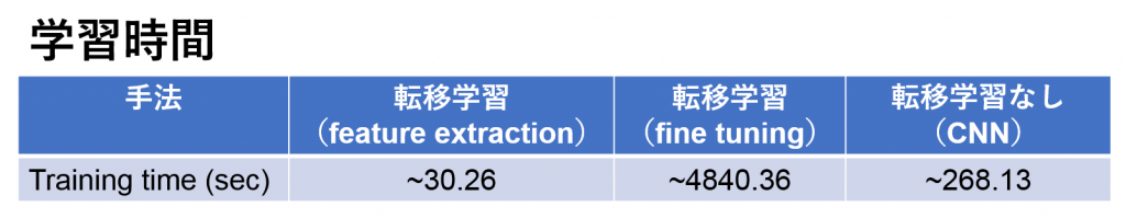
学習時間の比較

学習時間を比較してみました。今回の実験（小さいデータセット）では、Feature extractionのみの転移学習が一番早かったです。しかし、fine tuningを使うと、かなり時間がかかります。

音声の予測

上記の３つ学習モデルをテストしました。結果は下記になります。

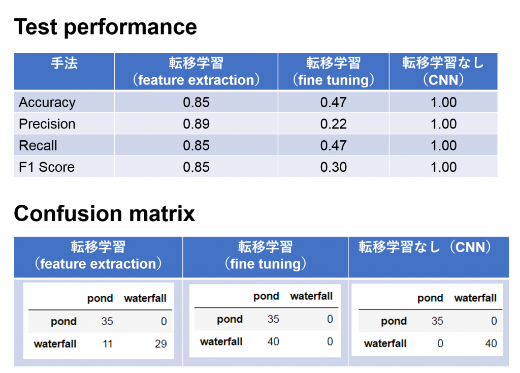
CNNの場合は100%の精度で池と滝の音が特定できました。転移学習では、feature extractionの場合、池の音はすべて特定できましたが、滝の音40サンプルの中で11個は外れました。また、今回のfine tuningは精度が出ませんでした。転移学習を使っても、きちんとチューニングを行わないと、逆に学習に悪影響があることがわかりました。残念です！

③ まとめと考察

今回は転移学習を紹介しました。例として、池と滝の音を分別してみました。簡単な実験ですが、転移学習（feature extractionのみ）の予測結果は85%くらい当たりました。転移学習で池と滝の識別するのは私の耳に勝てそうですが、みんなさんの耳にはまだ不十分かもしれません。

また、技術面だと、予想通りに、転移学習を利用すると、学習時間を節約できる可能性が見えました。しかし、転移学習（特にfine tuning）を利用すると学習に悪影響を与える可能性もあり、気をつけないといけないことがわかりました。

個人的には学習済モデルがどんどん出てきているので、転移学習の使い道が広がっていくのではないかと思います。

最後に

次世代システム研究室では、ビッグデータ解析プラットホームの設計・開発を行うアーキテクトとデータサイエンティストを募集しています。興味を持って頂ける方がいらっしゃいましたら、ぜひ 募集職種一覧からご応募をお願いします。

一緒に勉強しながら楽しく働きたい方のご応募をお待ちしております。